6Example 3 - constant-velocity 1D position tracking
Kalman filters are extensively used in navigation and other GPS-based systems. These can be either linear or nonlinear. In the latter case, one usually resorts to the extended Kalman, filter (EKF) that is designed to deal better with nonlinear state equations—see below.
Process noise design for \(Q\)
diagonal
constant velocity model
constant acceleration model
We begin with a very simple case of tracking a 1D position due to constant velocity motion, described by
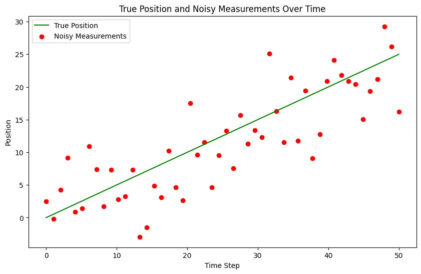
We begin by simulating the motion and generating noisy measurements of the position.
import numpy as npimport matplotlib.pyplot as plt# Set the random seed for reproducibilitynp.random.seed(42)# Simulate the ground truth position of the objecttrue_velocity =0.5# units per time stepnum_steps =50time_steps = np.linspace(0, num_steps, num_steps)true_positions = true_velocity * time_steps# Simulate the measurements with noisemeasurement_noise =5#1#0 # increase this value to make measurements noisiernoisy_measurements = true_positions + np.random.normal(0, measurement_noise, num_steps)# Plot the true positions and the noisy measurementsplt.figure(figsize=(10, 6))plt.plot(time_steps, true_positions, label='True Position', color='green')plt.scatter(time_steps, noisy_measurements, label='Noisy Measurements', color='red', marker='o')plt.xlabel('Time Step')plt.ylabel('Position')plt.title('True Position and Noisy Measurements Over Time')plt.legend()plt.show()
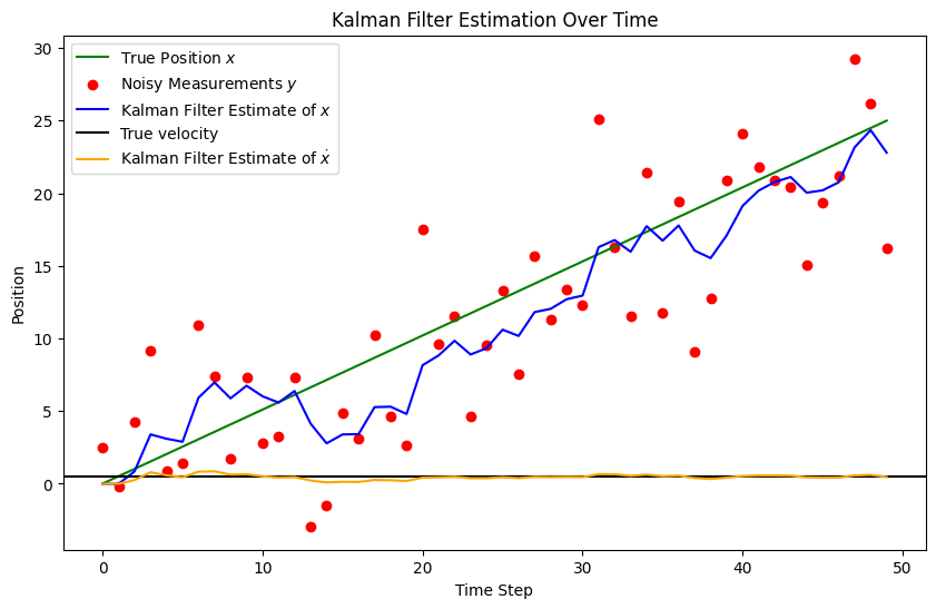
Now, we set up the inputs for the Kalman filter, run it, and plot the results of the estimation.
The process noise covariance matrix, \(Q,\) is taken here as
This form for \(Q\) can be derived from the discretization of a Wiener process, as shown in {cite}Sarkka2023. We will consider a more general case in Example 4, below.
sig_v = measurement_noisesig_w =0.1# np.sqrt(3) # process noise# Kalman Filter InitializationF = np.array([[1, 1], [0, 1]]) # State transition matrixH = np.array([[1, 0]]) # Measurement functionQ = np.array([[1, 0], [0, sig_w**2]]) # Process noise covarianceR = np.array([[sig_v**2]]) # Measurement noise covariancex0 = np.array([[0], [0]]) # Initial state estimateP0 = np.array([[1, 0], [0, 1]]) # Initial estimate covariance# Initialize the state estimate and covariancend =2T =50x_hat = np.zeros((T, nd, 1))P = np.zeros((T, nd, nd))x_hat[0] = x0P[0] = P0 #Qy = noisy_measurements# Run the Kalman filterfor t inrange(1, T):# Prediction step x_hat[t] = F @ x_hat[t-1] P[t] = F @ P[t-1] @ F.T + Q# Update step K = P[t] @ H.T @ np.linalg.inv(H @ P[t] @ H.T + R) x_hat[t] = x_hat[t] + K @ (y[t] - H @ x_hat[t]) P[t] = (np.eye(nd) - K @ H) @ P[t]
# Plot the true positions, noisy measurements, and the Kalman filter estimatestime_steps =range(T)estimated_positions = x_hat[:,0,:]estimated_velocities = x_hat[:,1,:]plt.figure(figsize=(10, 6))plt.plot(time_steps, true_positions, label='True Position $x$', color='green')plt.scatter(time_steps, noisy_measurements, label='Noisy Measurements $y$', color='red', marker='o')plt.plot(time_steps, estimated_positions, label='Kalman Filter Estimate of $x$', color='blue')plt.axhline(0.5,color='k',label='True velocity')plt.plot(time_steps, estimated_velocities, label='Kalman Filter Estimate of $\dot{x}$', color='orange')plt.xlabel('Time Step')plt.ylabel('Position')plt.title('Kalman Filter Estimation Over Time')plt.legend()plt.show()
Asch, Mark. 2022. A Toolbox for DigitalTwins: FromModel-Based to Data-Driven. Philadelphia, PA: Society for Industrial; Applied Mathematics. https://doi.org/10.1137/1.9781611976977.
Asch, Mark, Marc Bocquet, and Maëlle Nodet. 2016. Data Assimilation: Methods, Algorithms, and Applications. Philadelphia, PA: Society for Industrial; Applied Mathematics. https://doi.org/10.1137/1.9781611974546.
Calvello, Edoardo, Sebastian Reich, and Andrew M. Stuart. 2022. “Ensemble KalmanMethods: AMeanFieldPerspective.” arXiv (to appear in Acta Numerica 2025). http://arxiv.org/abs/2209.11371.
Carrillo, J. A., F. Hoffmann, A. M. Stuart, and U. Vaes. 2024a. “Statistical Accuracy of Approximate Filtering Methods.”https://arxiv.org/abs/2402.01593.
Dashti, Masoumeh, and Andrew M. Stuart. 2015. “The BayesianApproach to InverseProblems.” In Handbook of UncertaintyQuantification, edited by Roger Ghanem, David Higdon, and Houman Owhadi, 1–118. Cham: Springer International Publishing. https://doi.org/10.1007/978-3-319-11259-6_7-1.
Huang, Daniel Zhengyu, Jiaoyang Huang, Sebastian Reich, and Andrew M Stuart. 2022. “Efficient Derivative-Free Bayesian Inference for Large-Scale Inverse Problems.”Inverse Problems 38 (12): 125006. https://doi.org/10.1088/1361-6420/ac99fa.
Iglesias, Marco A, Kody J H Law, and Andrew M Stuart. 2013. “Ensemble Kalman Methods for Inverse Problems.”Inverse Problems 29 (4): 045001. https://doi.org/10.1088/0266-5611/29/4/045001.
Law, Kody, Andrew Stuart, and Konstantinos Zygalakis. 2015. Data Assimilation: AMathematicalIntroduction. Vol. 62. Texts in AppliedMathematics. Cham: Springer International Publishing. https://doi.org/10.1007/978-3-319-20325-6.
Sanita Vetra-Carvalho, Lars Nerger, Peter Jan van Leeuwen, and Jean-Marie Beckers. 2018. “State-of-the-Art Stochastic Data Assimilation Methods for High-Dimensional Non-Gaussian Problems.”Tellus A: Dynamic Meteorology and Oceanography 70 (1): 1–43. https://doi.org/10.1080/16000870.2018.1445364.
Särkkä, S., and L. Svensson. 2023. Bayesian Filtering and Smoothing. 2nd ed. Institute of Mathematical Statistics Textbooks. Cambridge University Press. https://doi.org/10.1017/9781108917407.
Wu, Jin-Long, Matthew E. Levine, Tapio Schneider, and Andrew Stuart. 2023. “Learning about Structural Errors in Models of Complex Dynamical Systems.”https://arxiv.org/abs/2401.00035.