import numpy as np
import matplotlib.pyplot as plt
from scipy import linalg
np.random.seed(1)


def Lorenz63(state, *args):
    """
    Parameters
    ----------
    state : array-like, shape (3,)
       Point of interest in three-dimensional space.
    *args (sigma, rho, beta) : float
       Parameters defining the Lorenz attractor.

    Returns
    -------
    state_dot : array, shape (3,)
       Values of the Lorenz attractor's derivatives at *state*.
    """
    sigma = args[0]
    rho = args[1]
    beta = args[2]
    x, y, z = state #Unpack the state vector
    f = np.zeros(3) #Derivatives
    f[0] = sigma * (y - x)
    f[1] = x * (rho - z) - y
    f[2] = x * y - beta * z
    return f

def RK4(rhs, state, dt, *args):

    k1 = rhs(state,         *args)
    k2 = rhs(state+k1*dt/2, *args)
    k3 = rhs(state+k2*dt/2, *args)
    k4 = rhs(state+k3*dt,   *args)

    new_state = state + (dt/6)*(k1 + 2*k2 + 2*k3 + k4)
return new_state13 Example 2: Lorenz63 system
In this example, we will concentrate on DA methods applied to the Lorenz systems of ordinary differential equations. These systems exhibit chaotic behavior and as such are considered as excellent toy models for complex phenomena, in particular for simulation of weather. The Lorenz-63 system is given by
\[\begin{align} \frac{\mathrm{d} x}{\mathrm{d} t} &= -\sigma(x-y), \nonumber \\ \frac{\mathrm{d} y}{\mathrm{d} t} &= \rho x-y-xz, \label{eq:lorenz} \\ \frac{\mathrm{d} z}{\mathrm{d} t} &= xy -\beta z, \nonumber \end{align}\] where \(x=x(t)\), \(y=y(t)\), \(z=z(t)\) and \(\sigma\) (ratio of kinematic viscosity divided by thermal diffusivity), \(\rho\) (measure of stability) and \(\beta\) (related to the wave number) are parameters.
Chaotic behavior is obtained when the parameters are chosen as
\[ \sigma = 10,\quad \rho=28,\quad \beta = 8/3. \]
Its solution is very sensitive to the parameters and the initial conditions and a small difference in these values can lead to a very different solution. This is the basis of its ill-posedness. This equation is a simplified model for atmospheric convection and is an excellent example of the lack of predictability. It is ill-posed in the sense of Hadamard. In fact the solution switches between two stable orbits, around the points
\[ \left(\sqrt{\beta(\rho-1)},\sqrt{\beta(\rho-1)},\rho-1\right), \quad \left(-\sqrt{\beta(\rho-1)},-\sqrt{\beta(\rho-1)},\rho-1\right).\]
# parameters Lorenz63
sigma = 10.0
rho  = 28.0
beta = 8.0/3.0
dt = 0.01
tm = 10
nt = int(tm/dt)
t  = np.linspace(0,tm,nt+1)
# initialize and solve
u0True = np.array([1,1,1]) # True initial conditions
#time integration
uTrue = np.zeros([nt+1,3])
uTrue[0,:] = u0True
for k in range(nt):
    uTrue[k+1,:] = RK4(Lorenz63,uTrue[k,:], dt, sigma, rho, beta)

# plot results
fig, ax = plt.subplots(nrows=3,ncols=1, figsize=(10,8))
ax = ax.flat

prop_cycle = plt.rcParams['axes.prop_cycle']
colors = prop_cycle.by_key()['color']

for k in range(3):
    ax[k].plot(t,uTrue[:,k], label='True', color = colors[k], linewidth = 3)
    ax[k].set_xlabel('t')

ax[0].set_ylabel('x(t)', labelpad=5)
ax[1].set_ylabel('y(t)', labelpad=-12)
ax[2].set_ylabel('z(t)')
fig.subplots_adjust(hspace=0.5)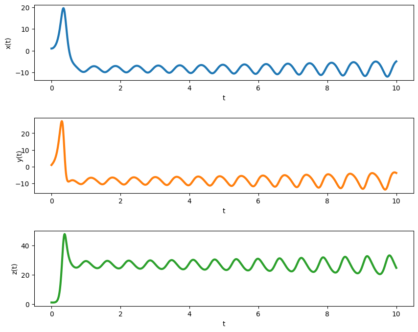
nt = 10000 # need longer time to see the attractor
uTrue = np.zeros([nt+1,3])
uTrue[0,:] = u0True

for k in range(nt):
    uTrue[k+1,:] = RK4(Lorenz63,uTrue[k,:], dt,sigma, rho, beta)

# Plot
ax = plt.figure(figsize=(10,8)).add_subplot(projection='3d')
ax.plot(*uTrue.T, lw=0.5)
ax.set_xlabel("$x(t)$")
ax.set_ylabel("$y(t)$")
ax.set_zlabel("$z(t)$")
ax.set_title("Lorenz Attractor")
plt.show()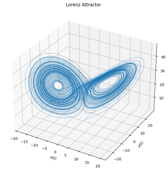
13.1 Ensemble KF for Data Assimilation
Here we will generalize the ensemble Kalman filter to take into account the possibility of sparse observations. This is usually the case in real-life systems, where observations are only available et fixed instants, and hence the filtering can only be applied at these times. Inbetween observations, the system evolves freely (without correction) according to its underlying state equation.
Suppose we have \(N_y\) measurements/observations at an interval of \(\delta t_y.\) This gives measurements for times \(t_0 \le t \le t_m,\) where \(t_m = N_m \delta t_m.\) This can be considered as the assimilation window. The system then evolves freely for \(t > t_m\) until some final forecast window time \(t_f.\) The state, or equation itself is simulated with a smaller \(\delta t\) and for a large number \(N_t\) steps, giving \(t_f = N_t \delta t.\) Usually, for real life systems, we will have
\[ \delta t_m \ge \delta t, \quad N_m \le N_t , \quad t_m \le t_f. \]
For code testing, we make the simplifying (unrealistic) academic assumption that
\[ \delta t_m = \delta t, \quad N_m = N_t, \quad t_f = t_m. \]
This implies the availabilty of measurements at each (and every) time step. Note that in many of the previous examples, this was indeed the case.
def enKF_Lorenz63_setup(dt, T, dt_m, T_m, sig_w, sig_v):
    """
    Prepare input (true state and observations) for the stochastic
    ensemble filter of the Lorenz63 system.

    Parameters:
        dt: time step for state evolution
        T:  time interval for state evolution
        dt_m: time interval between 2 measurements (can equal dt for dense observations)
        T_m: time interval for observations
        sig_w: state noise sd., cov. Q = sig_w**2 x np.eye(3)
        sig_v: measurement noise sd., cov. R = sig_v**2 x np.eye(3)
    """
    # parameters Lorenz63
    sigma = 10.0
    rho  = 28.0
    beta = 8.0/3.0
    dim_x = 3
    dim_y = 3
    # noise covariances
    Q  = sig_w**2 * np.eye(dim_x)
    R  = sig_v**2 * np.eye(dim_y)
    # measurement operator (identity here)
    def H(u):
        w = u
        return w

    # Solve system and generate noisy observations
    Nt = int(T/dt)     # number of time steps
    Nm = int(T_m/dt_m) # number of observations
    t = np.linspace(0, Nt, Nt+1) * dt # time vector (including 0 and T)
    ind_m = (np.linspace(int(dt_m/dt),int(T_m/dt),Nm)).astype(int) # obs. indices
    t_m = t[ind_m] # measurement time vector
    x0True = np.array([1.0, 1.0, 1.0]) # True initial conditions
    sqrt_Q = np.linalg.cholesky(Q) # noise std dev.
    sqrt_R = np.linalg.cholesky(R)
    # initialize (correctly!)
    xTrue = np.zeros([Nt+1, dim_x])
    xTrue[0, :] = x0True
    y = np.zeros((Nm, dim_y))
    km = 0 # index for measurement times
    y[0,:] = H(xTrue[0,:]) + sig_v * np.random.randn(dim_y)
    for k in range(Nt):
        w_k = sqrt_Q @ np.random.randn(dim_x)
        xTrue[k+1,:] = RK4(Lorenz63,xTrue[k,:], dt,sigma, rho, beta) #+ w_k
        if (km < Nm) and (k+1 == ind_m[km]):
            v_k = sqrt_R @ np.random.randn(dim_y)
            y[km,:]     = H(xTrue[k+1,:]) + v_k
            km = km + 1
    # plot state and measurements
    fig, ax = plt.subplots(nrows=3,ncols=1, figsize=(10,8))
    ax = ax.flat
    #t = T*dt
    for k in range(3):
        ax[k].plot(t,xTrue[:,k], label='True', linewidth = 3)
        ax[k].plot(t[ind_m],y[:,k], 'o', fillstyle='none', \
                   label='Observation', markersize = 8, markeredgewidth = 2)
        ax[k].set_xlabel('t')
        ax[k].axvspan(0, T_m, color='lightgray', alpha=0.4, lw=0)
    ax[0].legend(loc="center", bbox_to_anchor=(0.5,1.25),ncol =4,fontsize=15)
    ax[0].set_ylabel('x(t)')
    ax[1].set_ylabel('y(t)')
    ax[2].set_ylabel('z(t)')
    fig.subplots_adjust(hspace=0.5)

    return Q, R, xTrue, y, ind_m, Nt, Nm
Q, R, xTrue, y, ind_m, Nt, Nm = enKF_Lorenz63_setup(dt=0.01, T=10, dt_m=0.2, T_m =2, sig_w=0.001, sig_v=0.15)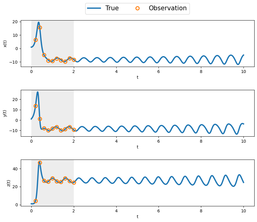
def enKF_Lorenz63_DA(x0, P0, Q, R, y, ind_m, Nt, Nm, Ne=10):
    """
    Run DA of the Lorenz63 system using the stochastic
    ensemble filter with sparse observations in the DA
    window, defined by time index set `ind_m`.

    Parameters:

    """
    # parameters Lorenz63
    sigma = 10.0
    rho  = 28.0
    beta = 8.0/3.0
    def Hx(u):
        w = u
        return w
    Nx     = x0.shape[-1]
    Ny     = y.shape[-1]
    enkf_m = np.empty((Nt+1, Nx))
    enkf_P = np.empty((Nt+1, Nx, Nx))
    X      = np.empty((Nx, Ne))
    Xf     = np.empty((Nx, Ne))
    HXf    = np.empty((Ny, Nx))

    X[:,:] = np.tile(x0, (Ne,1)).T  + np.linalg.cholesky(P0)@np.random.randn(Nx, Ne) # initial ensemble state
    P       = P0 # initial state covariance
    enkf_m[0, :]    = x0
    enkf_P[0, :, :] = P0

    i_m = 0 # index for measurement times

    for i in range(Nt):
        # ==== predict/forecast ====
        for e in range(Ne):
            w_i = np.linalg.cholesky(Q) @ np.random.randn(Nx)#, Ne)
            Xf[:,e] = RK4(Lorenz63, X[:,e], dt, sigma, rho, beta) + w_i # predict state ensemble
        mX = np.mean(Xf, axis=1)        # state ensemble mean
        Xfp = Xf - mX[:, None]          # state forecast anomaly
        P = Xfp @ Xfp.T / (Ne - 1)      # predict covariance
        # ==== prepare analysis step =====
        if (i_m < Nm) and (i+1 == ind_m[i_m]):
            HXf = Hx(Xf)                    # nonlinear observation
            mY = np.mean(HXf, axis=1)       # observation ensemble mean
            HXp = HXf - mY[:, None]         # observation anomaly
            S = (HXp @ HXp.T)/(Ne - 1) + R  # observation covariance
            K = linalg.solve(S, HXp @ Xfp.T, assume_a="pos").T  / (Ne - 1)  # Kalman gain
            # === perturb y and compute innovation ====
            ypert = y[i_m, :] +  (np.linalg.cholesky(R)@np.random.randn(Ny, Ne)).T
            d = ypert.T - HXf
            # ==== correct/analyze ====
            X[:,:] = Xf + K @ d          # update state ensemble
            mX = np.mean(X[:,:], axis=1) # state analysis ensemble mean
            Xap = X[:,:] - mX[:, None]   # state analysis anomaly
            P = Xap @ Xap.T / ( Ne - 1)  # update covariance
            i_m = i_m + 1
        else:
            X[:,:] = Xf  # when there is no obs, then state=forecast
        # ==== save ====
        enkf_m[i+1] = mX                # save KF state estimate (mean)
        enkf_P[i+1] = P                 # save KF error estimate (covariance)
    return enkf_m, enkf_P
# Initialize and run the analysis
sig_w = 0.0015
sig_v = 0.15
Q = sig_w**2 * np.eye(3) #* 1.e-6 # for comparison with DT
R = sig_v**2 * np.eye(3)
x0 = np.array([2., 3., 4.]) # a little off
sig_vv = 0.1
P0 = np.eye(3) * sig_vv**2 # Initial estimate covariance
Ne = 10
Xa, P = enKF_Lorenz63_DA(x0, P0, Q, R, y, ind_m, Nt, Nm, Ne=10)# Post-process and plot the results
# generate unfiltered state
Xb = np.empty((Nt+1, 3))
Xb[0,:] = x0
for i in range(Nt):
Xb[i+1,:] = RK4(Lorenz63, Xb[i,:], dt, sigma, rho, beta)
# plot state and measurements
t = np.linspace(0, Nt, Nt+1) * dt # time vector
T_m = 2.
fig, ax = plt.subplots(nrows=3,ncols=1, figsize=(10,8))
ax = ax.flat
for k in range(3):
ax[k].plot(t,xTrue[:,k], label='True')#, linewidth = 3)
ax[k].plot(t,Xa[:,k], '--', label='EnKF analysis')#, linewidth = 3)
ax[k].plot(t[ind_m],y[:,k], 'o', fillstyle='none', \
label='Observation')#, markersize = 8, markeredgewidth = 2)
ax[k].plot(t,Xb[:,k], ':', label='Unfiltered')#, linewidth = 3)
ax[k].set_xlabel('t')
ax[k].axvspan(0, T_m, color='lightgray', alpha=0.4, lw=0)
ax[0].legend(loc="center", bbox_to_anchor=(0.5,1.25),ncol =4,fontsize=15)
ax[0].set_ylabel('x(t)')
ax[1].set_ylabel('y(t)')
ax[2].set_ylabel('z(t)')
fig.subplots_adjust(hspace=0.5)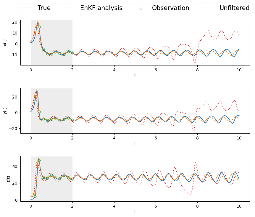
13.2 Conclusion
The ensemble Kalman filter, even with very sparse observations and a chaotic system, does an excellent job of
- tracking within the DA window,
- forecasting way beyond the window, whereas the unfiltered/unassimilated, freely evolving system deviates considerably, as is to be expected from the chaotic Lorenz system.
From \(t \approx 6,\) the KF starts to deviate very slightly, mostly a phase difference. However, in real situations, there will already be new measurements available by this time. Then the KF analysis will kick in again, and rectify the trajectory.