import matplotlib.pyplot as plt
import numpy as np
from scipy import linalg, stats
# we use Sarkka's utilities to streamline a bit...
from common_utilities import generate_pendulum, RandomState, rmse, plot_pendulum
# initialize
dt = 0.01  # time step
g  = 9.81  # gravitational acceleration

sig_w = 0.1          # process noise
sig_v = np.sqrt(0.1) # measurement noise

Q  = sig_w**2 * np.array([[dt ** 3 / 3, dt ** 2 / 2],
                          [dt ** 2 / 2, dt]])
R  = sig_v**2 * np.eye(1)

x_0 = np.array([1.5, 0.])10 Example 2 - tracking a noisy pendulum
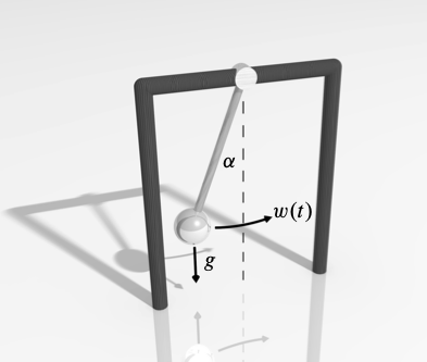
Consider the nonlinear ODE model for the oscillations of a noisy pendulum with unit mass and length \(L,\)
\[ \frac{\mathrm{d}^{2}\theta}{\mathrm{d} t^{2}}+\frac{g}{L}\sin\theta+w(t)=0 \]
where \(\theta\) is the angular displacement of the pendulum, \(g\) is the gravitational constant, \(L\) is the pendulum’s length, and \(w(t)\) is a white noise process. This is rewritten in state space form,
\[ \dot{\mathbf{x}}+\mathcal{M}(\mathbf{x})+\mathbf{w}=0, \]
where
\[ \mathbf{x}=\left[\begin{array}{c} x_{1}\\ x_{2} \end{array}\right]=\left[\begin{array}{c} \theta\\ \dot{\theta} \end{array}\right],\quad \mathcal{M}(\mathbf{x})=\left[\begin{array}{c} x_{2}\\ -\dfrac{g}{L}\sin x_{1} \end{array}\right],\quad \mathbf{w}=\left[\begin{array}{c} 0\\ w(t) \end{array}\right]. \]
Suppose that we have discrete, noisy measurements of the horizontal component of the position, \(\sin (\theta).\) Then the measurement equation is scalar,
\[ y_k = \sin \theta_k + v_k, \]
where \(v_k\) is a zero-mean Gaussian random variable with variance \(R.\) The system is thus nonlinear in state and measurement and the state-space system is of the general form seen above. A simple discretization, based on Euler’s method produces
\[\begin{align*} \mathbf{x}_{k} & =\mathcal{M}(\mathbf{x}_{k-1})+\mathbf{w}_{k-1}\\ {y}_{k} & = \mathcal{H}_{k}(\mathbf{x}_{k}) + {v}_{k}, \end{align*}\]
where
\[ \mathbf{x}_{k}=\left[\begin{array}{c} x_{1}\\ x_{2} \end{array}\right]_{k}, \quad \mathcal{M}(\mathbf{x}_{k-1})=\left[\begin{array}{c} x_1 + \Delta t x_{2}\\ x_2 - \Delta t \dfrac{g}{L}\sin x_{1} \end{array}\right]_{k-1}, \quad \mathcal{H}(\mathbf{x}_{k}) = [\sin x_{1}]_k . \]
The noise terms have distributions
\[ \mathbf{w}_{k-1}\sim\mathcal{N}(\mathbf{0},Q),\quad v_{k}\sim\mathcal{N}(0,R), \]
where the process covariance matrix is
\[ Q=\left[\begin{array}{cc} q_{11} & q_{12}\\ q_{21} & q_{22} \end{array}\right], \]
with components (see KF example for 2D motion tracking),
\[ q_{11}=q_{c}\frac{\Delta t^{3}}{3},\quad q_{12}=q_{21}=q_{c}\frac{\Delta t^{2}}{2},\quad q_{22}=q_{c}\Delta t, \]
and \(q_c\) is the continuous process noise spectral density.
For the first-order EKF—higher orders are possible—we will need the Jacobian matrices of \(\mathcal{M}(\mathbf{x})\) and \(\mathcal{H}(\mathbf{x})\) evaluated at \(\mathbf{x} = \mathbf{\hat{m}}_{k-1}\) and \(\mathbf{x} = \mathbf{\hat{m}}_{k}\) . These are easily obtained here, in an explicit form,
\[ \mathbf{M}_{\mathbf{x}}=\left[\frac{\partial\mathcal{M}}{\partial\mathbf{x}}\right]_{\mathbf{x}=\mathbf{m}}=\left[\begin{array}{cc} 1 & \Delta t\\ -\Delta t \dfrac{g}{L}\cos x_{1} & 1 \end{array}\right]_{k-1}, \]
and
\[ \mathbf{H}_{\mathbf{x}}=\left[\frac{\partial\mathcal{H}}{\partial\mathbf{x}}\right]_{\mathbf{x}=\mathbf{m}}=\left[\begin{array}{cc} \cos x_{1} & 0\end{array}\right]_k. \]
Results are plotted in Figure. We notice that despite the very noisy, nonlinear measurements, the EKF rapidly approaches the true state and then tracks it extremely well.
# Simulate trajectory and noisy measurements
random_state = RandomState(1)
steps = 500

timeline, states, observations = generate_pendulum(x_0, g, Q, dt, R, steps, random_state)
plot_pendulum(timeline, observations, states, "Trajectory")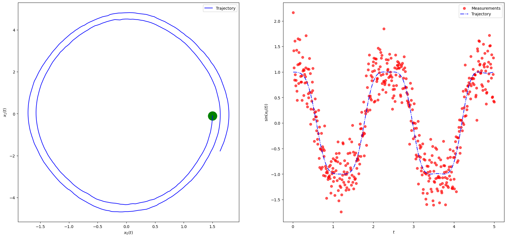
10.1 Extended Kalman Filter (EKF)
def extended_kalman_filter(m_0, P_0, g, Q, dt, R, observations):
    n = m_0.shape[-1]
    steps = observations.shape[0]

    ekf_m = np.empty((steps, n))
    ekf_P = np.empty((steps, n, n))

    m = m_0[:]
    P = P_0[:]

    for i in range(steps):
        y = observations[i]

        # Jacobian of the dynamic model function
        Df = np.array([[1.,                     dt],
                      [-g * dt * np.cos(m[0]), 1.]])

        # Predicted state distribution
        m = np.array([m[0] + dt * m[1],
                      m[1] - g * dt * np.sin(m[0])])
        P = Df @ P @ Df.T + Q

        # Predicted observation
        h  = np.sin(m[0])
        Dh = np.array([[np.cos(m[0]), 0.]])
        S = Dh @ P @ Dh.T + R

        # Kalman Gain
        K = linalg.solve(S, Dh @ P, assume_a="pos").T
        m = m + K @ np.atleast_1d(y - h)
        P = P - K @ S @ K.T

        ekf_m[i] = m
        ekf_P[i] = P
    return ekf_m, ekf_P
# initialize state and covariance
m_0 = np.array([1.6, 0.]) # Slightly off
P_0 = np.array([[0.1, 0.],
[0., 0.1]])
ekf_m, ekf_P = extended_kalman_filter(m_0, P_0, g, Q, dt, R, observations)
plot_pendulum(timeline, observations, states, "Trajectory", ekf_m, "EKF Estimate")
rmse_ekf = rmse(ekf_m[:, :1], states[:, :1])
print(f"EKF RMSE: {rmse_ekf}")EKF RMSE: 0.10306106181239276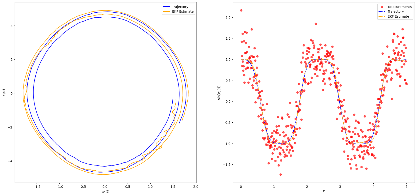
# plot covariances
plt.plot(timeline, ekf_P[:,0,0], timeline,ekf_P[:,1,1] )
plt.legend(['P(1,1)', 'P(2,2)'])
plt.show()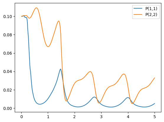
10.2 Extended Smoother
def extended_smoother(ekf_m, ekf_P, g, Q, dt):
    steps, M = ekf_m.shape

    rts_m = np.empty((steps, M))
    rts_P = np.empty((steps, M, M))

    m = ekf_m[-1]
    P = ekf_P[-1]

    rts_m[-1] = m
    rts_P[-1] = P

    for i in range(steps-2, -1, -1):
        filtered_m = ekf_m[i]
        filtered_P = ekf_P[i]

        Df = np.array([[1., dt],
                      [-g * dt * np.cos(filtered_m[0]), 1.]])

        mp = np.array([filtered_m[0] + dt * filtered_m[1],
                       filtered_m[1] - g * dt * np.sin(filtered_m[0])])
        Pp = Df @ filtered_P @ Df.T + Q

        # More efficient and stable way of computing Gk = filtered_P @ A.T @ linalg.inv(Pp)
        # This also leverages the fact that Pp is known to be a positive definite matrix (assume_a="pos")
        Gk = linalg.solve(Pp, Df @ filtered_P, assume_a="pos").T

        m = filtered_m + Gk @ (m - mp)
        P = filtered_P + Gk @ (P - Pp) @ Gk.T

        rts_m[i] = m
        rts_P[i] = P

    return rts_m, rts_P
rts_m, rts_P = extended_smoother(ekf_m, ekf_P, g, Q, dt)
plot_pendulum(timeline, observations, states, "Trajectory", rts_m, "Extended Smoother Estimate")
rmse_erts = rmse(rts_m[:, :1], states[:, :1])
print(f"KF RMSE: {rmse_ekf}")
print(f"ERTS RMSE: {rmse_erts}")KF RMSE: 0.10306106181239276
ERTS RMSE: 0.027612762479911554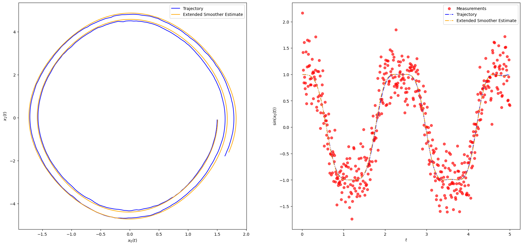
10.3 Conclusions on Extended Kalman Filters
The pros and cons of the EKF are:
Pros:
- Relative simplicity, based on well-known linearization methods.
- Maintains the simple, elegant, and computationally efficient KF update equations.
- Good performance for such a simple method.
- Ability to treat nonlinear process and observation models.
- Ability to treat both additive and more general nonlinear Gaussian noise.
Cons:
- Performance can suffer in presence of strong nonlinearity because of the local validity of the linear approximation (valid for small perturbations around the linear term).
- Cannot deal with non-Gaussian noise, such as discrete-valued random variables.
- Requires differentiable process and measurement operators and evaluation of Jacobian matrices, which might be problematic in very high dimensions.
In spite of this, the EKF remains a solid filter and remains the basis of most GPS and navigation systems.
10.4 References
- K. Law, A Stuart, K. Zygalakis. Data Assimilation. A Mathematical Introduction. Springer. 2015.
- M. Asch, M. Bocquet, M. Nodet. Data Assimilation: Methods, Algorithms and Applications. SIAM. 2016.
- M. Asch. A Toobox for Digital Twins. From Model-Based to Data-Driven. SIAM. 2022
- S. Sarkka, L. Svensson. Bayesian Filtering and Smoothing, 2nd ed., Cambridge University Press. 2023.