Uncertainty
In practice some of the scheduling parameters may be uncertain. The exact duration of an activity, for instance, might not be known at the beginning of the project. Similarly, the number of available resources is another parameter that may not be known before project execution. These uncertainties may be due to different sources, including estimation errors, unforeseen (weather) conditions, late “delivery” (unavailability) of some required resources, unpredictable incidents such as machine breakdown or worker accidents, etc.
Stochastic, multistage programming
Background
Stochastic programming/optimization (optimal decision-making under uncertainty) is the part of mathematical programming and operations research that studies how to incorporate uncertainty into decision problems. Stochastic programs are primarily about transient decision making.
Some decisions must be made today, but important information will not be available until after the decision is made.
An information stage (normally simply called “stage”) is the most important concept that distinguishes stochastic programming. A stage is a point in time where decisions are made within a model. Stages define the boundaries of time intervals. Stages sometimes follow naturally from the problem setting and sometimes are modeling approximations.
The starting point of a stochastic program is the present situation. The model is intended to tell us what to do in light of our goals, constraints, and resources. We then ask what we should do. We are not asking what to do in all possible situations, just what to do based on our present state.
- An inherently two-stage model is a model where the first decision is a major long-term decision, whereas the remaining stages represent the use of this investment. In these cases, mathematically speaking, the first stage will look totally different from the remaining stages, which will all look more or less the same. This is a very important class of models, possibly the most important one for stochastic programming.
- In inherently multistage models, all stages are of the same type. We face random resource availability, energy prices, unexpected maintenance, etc. We should not confuse information stages with time periods. Stages model the flow of information; time periods represent the ticking of the clock in a model. Stages, on the other hand, are points in time where we make decisions in the model after having learned something new.
Finding a good trade-off between time periods and stages is often crucial when modeling, as it has consequences for model quality, data collection, and solvability of the model.
In the long run we are all dead. (J.M. Keynes)
In other words, one should not wait too long before taking a decision.
Mathematical Formulation
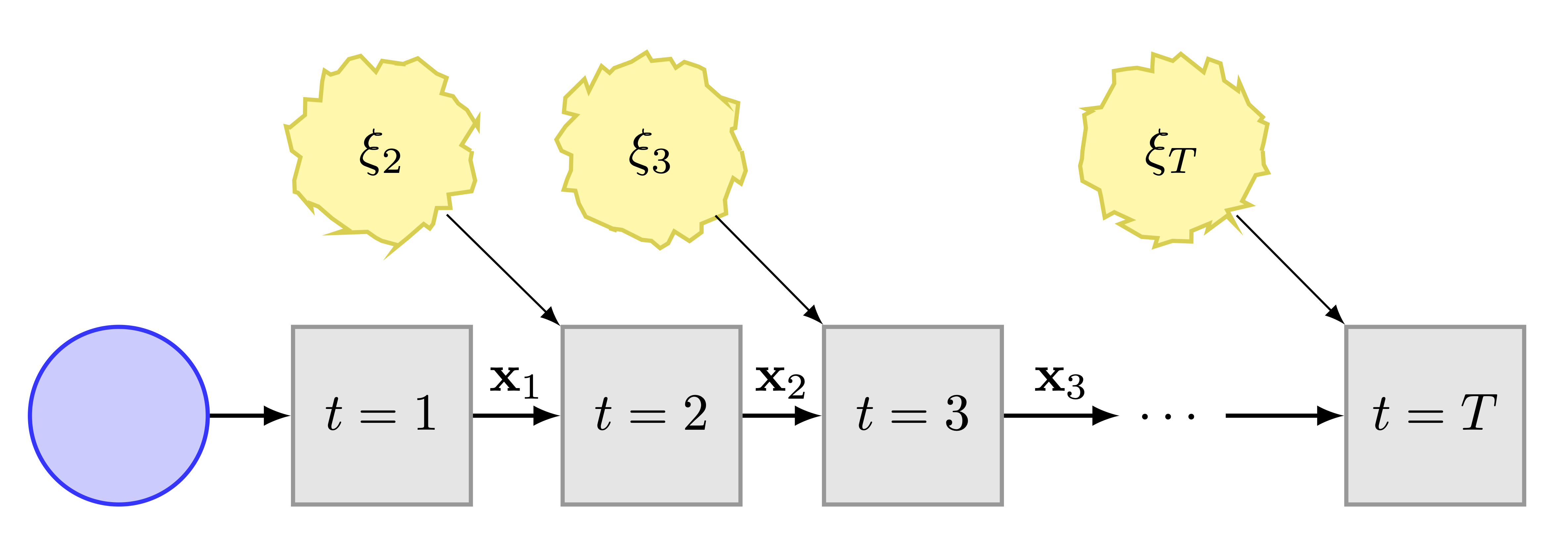
In the Figure we depict a generic multistage decision process with state \(\mathbf{x}_t\) that evolves over time, starting at stage \(t=1,\) and then receives uncertain, exogenous inputs, \(\xi_2, \xi_3, \ldots, \xi_T,\) at given stages \(t = 2,3,\ldots, T.\) At stage 1, a here-and-now (deterministic) decision is taken. The subsequent sequence of wait-and-see decision functions \({\mathbf{x}_t(\xi_t)}_{t\in [T]}\) constitutes a policy, \(\pi.\) The policy thus obtained, provides a decision rule for all stages \(t \in [T].\) The aim of the decision process (stochastic multistage optimization) is then to compute an optimal policy for a given objective and subject to constraints.
We will describe in detail the two-stage problem, since the multistage is a straightforward generalisation. In the stochastic setting, we can naturally classify \(x\in\mathscr{X}\) as the first-stage decision variables, since the initial facilities1 are fixed and \(y\in\mathbb{R}^{\left|\mathscr{A}\right|\times\left|\mathscr{K}\right|}\) as the second-stage decision variables, since the job-flow operating conditions are uncertain over time.
1 Data centers, HPC centers, networks.
The two-stage stochastic linear program (Birge and Louveaux 2011), (Shapiro et al. 2009) is then
\[\begin{align} \label{eq:2stage} \min_{x\in\mathscr{X}} & \,\,c^{\top}x + \mathrm{E}\left[Q(x;\xi)\right], \end{align}\] where \(Q(x;\xi)\) is the optimal value of the second-stage problem \[\begin{align*} \min_{y\ge0} & \,\,q^{\top}y\\ \textrm{s.t.} & \,\,Ny=0,\\ & Cy\ge d,\\ & Sy\le s,\\ & Ry\le Mx, \end{align*}\] where \(d\) is the (uncertain) resource demand, \(s\) is the (uncertain) resource supply, the random vector \(\xi=(q,d,s,R,M)\) and \(y=y(\xi).\) The expectation is taken with respect to the joint probability distribution function2 of \(\xi.\) In the terminology of state-space, we can consider \(x\) as the state variable, and \(y\) as the control variable.
2 Either continuous or discrete, it is derived either from theory or observations, or both.
To treat the occurrence of infeasibility, where the first-stage solution does not satisfy the second-stage constraints, e.g. \(Cy\ngeqslant d,\) we introduce a recourse action \(z\) that supplies the deficit \(d-Cy\) at some penalty cost. Then the second-stage problem becomes \[\begin{align*} \min_{y\ge0} & \,\,q^{\top}y+h^{\top}z\\ \textrm{s.t.} & \,\,Ny=0,\\ & Cy+z\ge d,\\ & Sy\le s,\\ & Ry\le Mx, \end{align*}\] where \(h\) represents the vector of (positive) recourse costs.
In the multistage case, we will have a succession of recourse stages, yielding the multistage program (Powell 2022),
\[ \min_{\pi \in \Pi} \mathrm{E} \left[ \sum^{T}_{t=1} \gamma^{t-1} f_t(x_t;\xi_t) \right], \] subject to \[ x_t \in \mathcal{X}_t(x_{t-1};\xi_{t-1}), \quad t=1 \ldots, T, \] where \(\pi\) is a policy, \(\gamma\) is a discount factor, \(f_t\) is a cost function, \(x_t\) is a decision and \(\mathcal{X}_t\) are the constraints. A policy is, by definition, a method that optimizes the objective. For example, in Google maps, the policy is to decide whether to turn left or right by optimizing over the time required to transverse the next link in the network plus the remaining time to get to the destination.
Note that there are various forms of minimization in stochastic scheduling. Whenever an objective function has to be minimized, it has to be specified in what sense the objective has to be minimized.
- Expectation sense is the crudest form of optimization, e.g., one wishes to minimize (a function of) the expected makespan, that is \(\mathrm{E}\left[f\left(C_{\mathrm{max}}\right)\right],\) and find a policy under which the expected makespan is smaller than the expected makespan under any other policy.
- Stochastic sense is a stronger form of optimization. If a schedule or policy minimizes \(f\left(C_{\mathrm{max}}\right)\) stochastically, then the makespan under the optimal schedule or policy is stochastically (in probability, or in law) less than the makespan under any other schedule or policy.
Chance Constraints
When the uncertainty is in the constraints, we can ensure that they hold with a certain probability. Suppose the constraints are of the form \[ A(z) x \le b(z) , \] where \(x\) is the decision variable and \(z\) is the random variable. Then the chance constraint can be \[ \mathrm{P} \left( a_i(z)^{\top} x - b_i(z) \le 0, \; \forall \; i=1,\ldots, m \right) \ge 1 - \epsilon \] for some \(\epsilon \in (0,1).\)
Risk Measures
Risk measures attempt to combine the two approaches: expectations, and probabilities of constraint violations. One example is given by \[ \max_{x\ge 0} \mathrm{E}_z f(x,z) - \kappa \mathrm{Var} \left( f(x,z) \right), \] where \(\kappa\) is a risk aversion parameter. The larger the value of \(\kappa,\) the more the optimization problem tries to find a solution with minimal variance, or less risk.
A risk measure \(\rho\) combines the expected value \(\mathrm{E}_z f(x,z)\) with another scalar term, called dispersion measure, which measures the uncertainty of the outcome.
The most common risk measures are:
- The mean-variance model, \[ \rho(Z) = \mathrm{E}(Z) - \kappa \mathrm{Var} (Z) . \]
- The value-at-risk (VaR), \[\rho(Z) = \mathrm{E}(Z) - \kappa \mathrm{VaR}_{\alpha} (Z),\] where \[\mathrm{VaR}_{\alpha} (Z) = \inf \{ t \colon \mathrm{P}(Z \le t ) \ge \alpha \} .\]
- The conditional value-at-risk (CVaR), \[\rho(Z) = \mathrm{CVaR}_{\alpha} (Z),\] where \[\mathrm{CVaR}_{\alpha} (Z) = \mathrm{E} \{ Z \vert Z \ge \mathrm{VaR}_{\alpha} (Z) \} .\]
- Exponential risk aversion, \[\rho(Z) = \inf_{\gamma > 0} \frac{1}{\gamma} \log \mathrm{E} \left( \exp(\gamma Z) \right). \]
Note that \(\mathrm{VaR}_{\alpha} (Z)\) can be rewritten as \(\mathrm{P} (Z \le \epsilon ) \ge \alpha.\) Finally, selecting the “right” function \(\rho\) depends on the modeling and optimization goals one has in mind.
Robust Optimization
In addition to the above two approaches—stochastic optimization and risk measures—there is a third approach, robust optimization, which is based on a worst-case analysis. we want the optimal solution to perform “the best possible,” assuming that the unknown problem parameters can always turn out to be “the worst possible.”
\[\begin{align*} \min & \sup_{z \in Z} \left[(c+Cz)^{\top} x \right] \\ \textrm{s.t.} & \quad (a_i + A_i z)^{\top} x \le b_i +b_i^{\top} Z, \, i=1,\ldots,m, \, \forall z \in Z,\\ & \quad x\in \mathbb{R}^n , \end{align*}\] where \(Z\) is the uncertainty set, and any single element \(z \in Z\) is a scenario.
A typical pattern emerges when comparing the solution between average-case stochastic optimization and robust optimization. The robust solution’s “range” of values is narrower, both in the best- and worst-situation sense, and it gives stabler profit relations. This comes, however, at the expense of having worse performance in an “average” scenario.
You can expect to observe this kind of phenomenon very often whenever you need to solve a problem under uncertainty and are unsure whether the worst-case or average-case performance should be optimized. The degree of trade-off can help you make the right decision.