Linear methods for classification
When confronted with a machine learning (ML) problem, one should always attempt linear methods before resorting to nonlinear ones. This is a general rule, whose major interest is to reach a better bias-variance tradeoff, and thus enhance the predictive power of your ML model–even if this is at the cost of slightly degraded accuracy.
For classification, there are three methods that should be tested, before using the classical SVM or random forest approaches. These are:
- Logistic regression.
- Linear discriminant analysis (LDA).
- Naive Bayes.
The last method, Naive Bayes, is covered in the book. This post will complete the first two.
Logistic Regression
In spite of its name, this is actually a classification method. The reasons for its popularity are:
- easy to implement and deploy
- easy to interpret
- very efficient training
- very fast classification of new data
- can provide information on the inportance of feautures
There are, however, three limitations.
- a linear hypothesis where the odds (see below) are linearly dependent on the predictors;
- the frontier between 2 classes is linear;
- only valid for binary classification, i.e. cases where there are only two classes.
Suppose that we have a binary response, yes or no, malignant or benign, sick or healthy, alive or dead… taking the value 0 or 1. And that we want to model the response
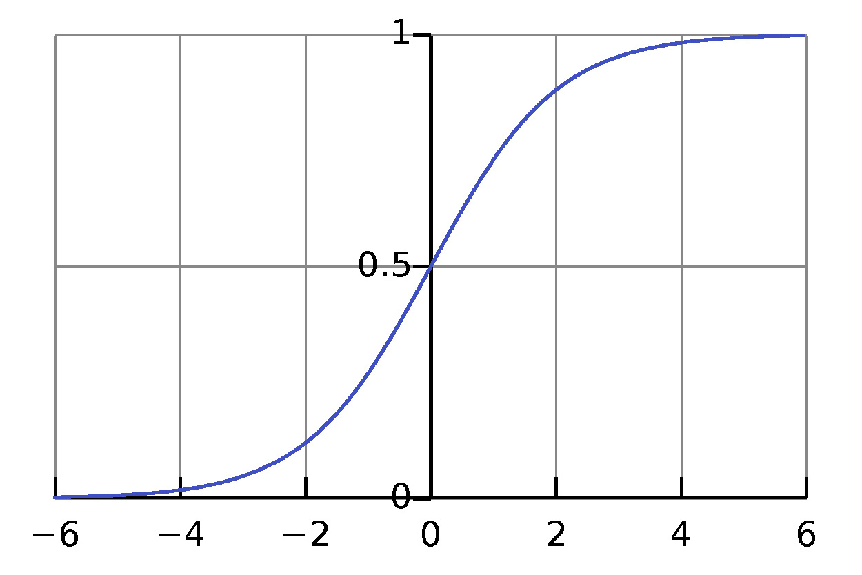
\[p(X) \doteq P(Y=1 \mid X).\]The logistic function that maps any interval into \([0, 1]\) is an excellent descriptor, where
\[p(X) = \frac{e^X}{1+e^X} = \frac{1}{1+e^{-X}}\]
Suppose now that we have a linear model for \(X\) of the form
\[\beta_0 + \beta_1 X ,\]then the logistic function becomes
\[p(X)=\frac{e^{\beta_{0}+\beta_{1}X}}{1+e^{\beta_{0}+\beta_{1}X}}=\frac{1}{1+e^{-(\beta_{0}+\beta_{1}X)}}\]and so
\[\frac{p(X)}{1-p(X)}=e^{\beta_{0}+\beta_{1}X}.\]But the LHS is just the odds ratio, so taking logaritms of this relation
\[\log\frac{p(X)}{1-p(X)}=\beta_{0}+\beta_{1}X\]we see that the so-called logit function is a linear function. We conclude that an increase of one unit in \(X\) produces an increase of \(\beta_{1}\) units in \(p(X).\) The coefficients \(\beta_{0}, \beta_{1}\) are estimated by a maximum likelihood (ML) method (as opposed to a least-squares for linear regression).
Finally, a prediction for a new, unseen value of \(X\) is given by
\[\hat{p}(X)=\frac{e^{\hat{\beta_{0}}+\hat{\beta_{1}}X}}{1+e^{\hat{\beta_{0}}+\hat{\beta_{1}}X}}=\frac{1}{1+e^{-(\hat{\beta_{0}}+\hat{\beta_{1}}X)}},\]where \(\hat{\beta_{0}}, \hat{\beta_{1}}\) are the ML estimates. The model can be extended to several predictors \(X_1, X_2, \dots, X_p,\) but not to more than 2 classes.
Here is an example of the use of logistic regression to predict Default as a function of Budget in a loan-rating analysis.

LDA
Linear discriminant analysis extends logistic regression to the case where we have more than two classes. We saw that LR models the conditional probability
\[P(Y=k\mid X=x)\]for 2 classes, based on the logistic function. For several classes, we need to model the distriution of the predictors separately for each class, and then use Bayes’ Law to compute the desired conditionals
\[P(Y=k\mid X=x)=\frac{\pi_{k}f_{k}(x)}{\sum_{l=1}^{K}\pi_{l}f_{l}(x)},\]where
- \(\pi_{k}\) is the prior probability of class \(k=1,\ldots,K\)
- \(f_{k}(x)=P(X=x\mid Y=k)\) is the likelihood
- \(p_{k}(x)=P(Y=k\mid X=x)\) is the posterior probability that the observation is of class \(k\) given the value of the predictor \(X=x\)
The likelihood is taken as Gaussian for each class, with equal variance
\[f_{k}(x)\sim\mathcal{N}(\mu_{k},\sigma).\]This gives the theoretical class frontier, known as the Bayes classifier,
\[\delta_{k}(x)=x\frac{\mu_{k}}{\sigma^{2}}-\frac{\mu_{k}^{2}}{2\sigma^{2}}+\log\pi_{k},\]also called the discriminant function, linear in \(x.\) Then we simply affect each observation to the class \(k\) for which this value is maximal. Finally, the LDA classifier is the approximation
\[\hat{\delta}_{k}(x)=x\frac{\hat{\mu}_{k}}{\hat{\sigma}^{2}}-\frac{\hat{\mu}_{k}^{2}}{2\hat{\sigma}^{2}}+\log\hat{\pi}_{k},\]where
- the estimated prior \(\hat{\pi}_{k}=n_{k}/n\)
- the estimated mean \(\hat{\mu_{k}}=(1/n_{k})\sum_{i:y_{i}=k}x_{i}\)
- the estimated variance \(\hat{\sigma}^{2}=1/(n-K)\sum_{k=1}^{K}\sum_{i:y_{i}=k}\left(x_{i}-\mu_{k}\right)^{2}\)
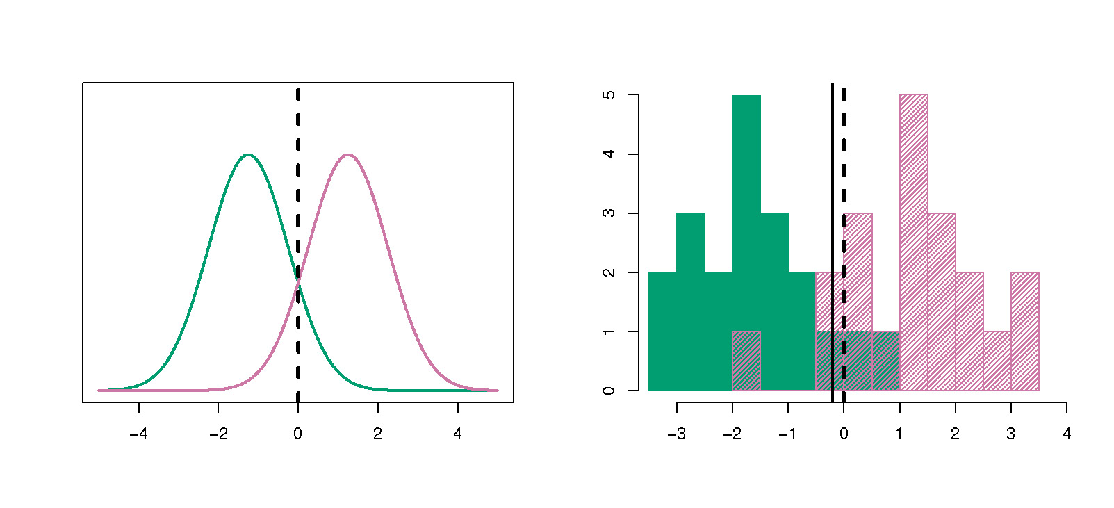
Here is an illustration of LDA for classifying 2 distributions.
